The Hamming Code

This is the first in a series of blog posts exploring the compilation of quantum algorithms to fault-tolerant architectures. We will

1. begin with the classical Hamming code,
2. extend it to the quantum Steane code,
3. learn about compilations of $T$-gates via magic state distillation,
4. reproduce key papers describing fault-tolerant compilation, and
5. explore methods to optimize the implementation of quantum simulation algorithms on early fault-tolerant devices

The series will focus on specifics (specific code, specific decoder, specific algorithm), and will aim to build intuition through numerical experiments.

In this post, I will give an overview of the $[[7,4,3]]$ Hamming code.

Definition of the code

The $[[n,k,d]]$ notation is a common short hand to describe an error-correcting code with $n$ physical bits encoding $k$ logical bits with a distance of $d$. The notion of distance in error-correcting codes is defined later in the notes.

In the $[[7,4,3]]$ code, we have 4 data bits (often called the message), combined with 3 parity bits to form 7-bit codewords. The mapping between messages and codewords is called an encoding, while the vector space generated by the codewords is called the codespace.

The codespace must obey a set of parity conditions. These parity conditions completely determine the Hamming code. For the $[[7,4,3]]$ code, the parity conditions are:

where all sums are modulo 2.

Since the codewords have 7 bits and must satisfy 3 independent constraints, there are $2^{7-3}=16$ codewords (we prove this below), which is also the number of 4-bit messages. So each message can be uniquely identified with a codeword.

Parity check and generator matrices

The three parity constraints can be expressed in terms of a parity check matrix:

A valid codeword $x$ then satisfies: $Hx^T=0$, where $0$ is the vector of 3 zeros. The codespace is, therefore, simply the kernel of the parity check matrix.

The dimension of the kernel follows from the rank-nullity theorem:

Since $H$ has 3 linearly independent rows, its rank is 3 and its nullity is 4, which confirms the previous claim that the codespace is 4 dimensional.

We can easily find a basis for the codespace by computing the kernel of $H$.

import numpy as np
import galois

GF2 = galois.GF(2)

# parity check matrix
H = np.array([
    [1, 0, 1, 0, 1, 0, 1],
    [0, 1, 1, 0, 0, 1, 1],
    [0, 0, 0, 1, 1, 1, 1],
])
H = GF2(H)

# generator matrix is null_space of H
G = H.null_space()
print(f'GH^T = {G @ H.T}')

The kernel is a $7\times 4$ matrix, $G$, satisfying $GH^T=0 \Rightarrow HG^T=0^T$, where $0$ represents the $4\times 3$ matrix of zeros. $G$ is also called the generator matrix since it is used to generate codewords for a given message, $m$. Let $x = mG$. We will show that $x$ a valid codeword:

Therefore, given the parity check matrix, one can compute the kernel and use it as an encoding map.

# encoding a message into a codeword
m = np.array([1, 0, 0, 1])
m = GF2(m)
x = m @ G

print(f'codeword = {x}')
print(f'Hx^T = {H @ x.T}')

For the $[[7,4,3]]$ Hamming code, the generator matrix is:

Error correction

Suppose we have encoded a message into a codeword $x$. Some time passes and we want to check if any bit-flip has occurred, and if so, correct the error. We can do this by simply checking the parity constraints: $Hx^T=0$.

The $[[7,4,3]]$ Hamming code can correct a single bit flip on any of its 7 bits. To see this, suppose the codeword $x$ has turned to $y=x+e$, where $e$ is a vector with $0$ everywhere and $1$ at the bit that has flipped. We would like to discover $e$ given $y$.

First we extract the syndrome, $Hy^T=He^T\equiv s$. Note that $s$ has 3 bits. So, we can have 7 distinct syndromes (aside from $s=0$). Each syndrome tells us a specific combination of parity constraints have been violated, which corresponds to a bit-flip on one of the 7 bits.

How do we decode this syndrome? Note that $s=He^T$ simply picks out the column of $H$ corresponding to the bit that has flipped. So, for instance, if the 3rd bit has flipped, $s$ is going to be $110$. Since there is a one-to-one mapping between syndromes and bit-flip locations, we can decode syndromes by using $H$ as a lookup table, and then correct the error by flipping the errant bits back.

# flip a bit
xp = x + GF2([0, 0, 0, 1, 0, 0, 0])

# extract syndrome
s = H @ xp.T
print(f'syndrome = {s}')

# decode syndrome
flipped_loc = np.where((H.T == s).all(axis=1))[0][0]
print(f"bit {flipped_loc} flipped")

# correct codeword
xp[flipped_loc] = GF2(1) - xp[flipped_loc]
remaining_error = np.linalg.norm(xp-x)
print(f"remaining error = {remaining_error}")

Error detection and code distance

What happens if 2 bits flip simultaneously? The syndrome $s$ is not $0$ so we can still detect that such an error. However, since there are only $8$ unique syndromes, and $7$ choose $2$ such events, there is no way to decode the syndrome, and any correction we perform might end up making matters worse.

# detection but no correction
xp = x + GF2([0, 0, 0, 1, 0, 0, 1])
s = H @ xp.T
print(f'syndrome = {s}')

# decode syndrome
flipped_loc = np.where((H.T == s).all(axis=1))[0][0]
print(f"bit {flipped_loc} flipped")

# correct codeword
xp[flipped_loc] = GF2(1) - xp[flipped_loc]
remaining_error = np.linalg.norm(xp-x)
print(f"remaining error = {remaining_error}")

What about 3 simultaneous bit flips? Looking at the generator matrix, we note that 3 bit flips are sufficient to convert the second codeword to the third. This means that 3 simultaneous bit flips could occur, and $Hy^T$ would still give $0$. Therefore, we cannot even detect some of the 3 bit flip events.

# cannot even detect
xp = x + GF2([0, 0, 1, 1, 0, 0, 1])
s = H @ xp.T
print(f'syndrome = {s}')

remaining_error = np.linalg.norm(xp-x)
print(f"remaining error = {remaining_error}")

# distance of code
d = min(sum(g) for g in np.array(G))
print(f'distance = {d}')

The distance of a code is defined as the minimum number of errors that can turn one codeword into another. We can work it out formally:

where $X$ is the codespace and $\lvert\cdot\rvert_H$ is the Hamming weight. In the second line we used the fact that the difference of two codewords is also a codeword, and in the last line we used the fact that the minimum Hamming weight of a row in $G$ is 3.

Break-even

Suppose each bit has some probability of flipping. This is called the physical error rate. Consider building a $[[7,4,3]]$ Hamming code from such bits. For low physical error rate, we will only ever see single bit flips, which the Hamming code can correct. However, as the physical error rate increases, more and more bits begin flipping simultaneously, and the error correction cycle fails. The rate at which error correction fails is called the logical error rate. As the physical error rate increase, at some point our encoding makes matters worse rather than better.

We can study the break-even below which the encoding is helpful by simulating the error correction protocol:

def cycle(x, p):
    err = GF2([1 if np.random.rand() < p else 0 for _ in range(7)])
    xp = x + err
    s = H @ xp.T

    flipped_loc = np.where((H.T == s).all(axis=1))[0]
    if len(flipped_loc) > 0:
        flipped_loc = flipped_loc[0]
        xp[flipped_loc] = GF2(1) - xp[flipped_loc]
    remaining_error = np.linalg.norm(xp-x)
    return remaining_error != 0        

num_cycles = 1000
reps = 10
pp_opts = np.logspace(-3, -0.1, 20)
pl_means = []
pl_stds = []
for pp in pp_opts:
    pl_list = []
    for _ in range(reps):
        pl = sum([cycle(x, pp) for _ in range(num_cycles)])/num_cycles
        pl_list.append(pl)

    pl_means.append(np.mean(pl_list))
    pl_stds.append(np.std(pl_list))

breakeven = 0.0
for pp, pl in zip(pp_opts, pl_means):
    if pl > pp:
        breakeven = pp
        break
print(f"break-even point = {breakeven}")

The simulation shows that the break-even point of the [[7,4,3]] Hamming code is approximately 0.07: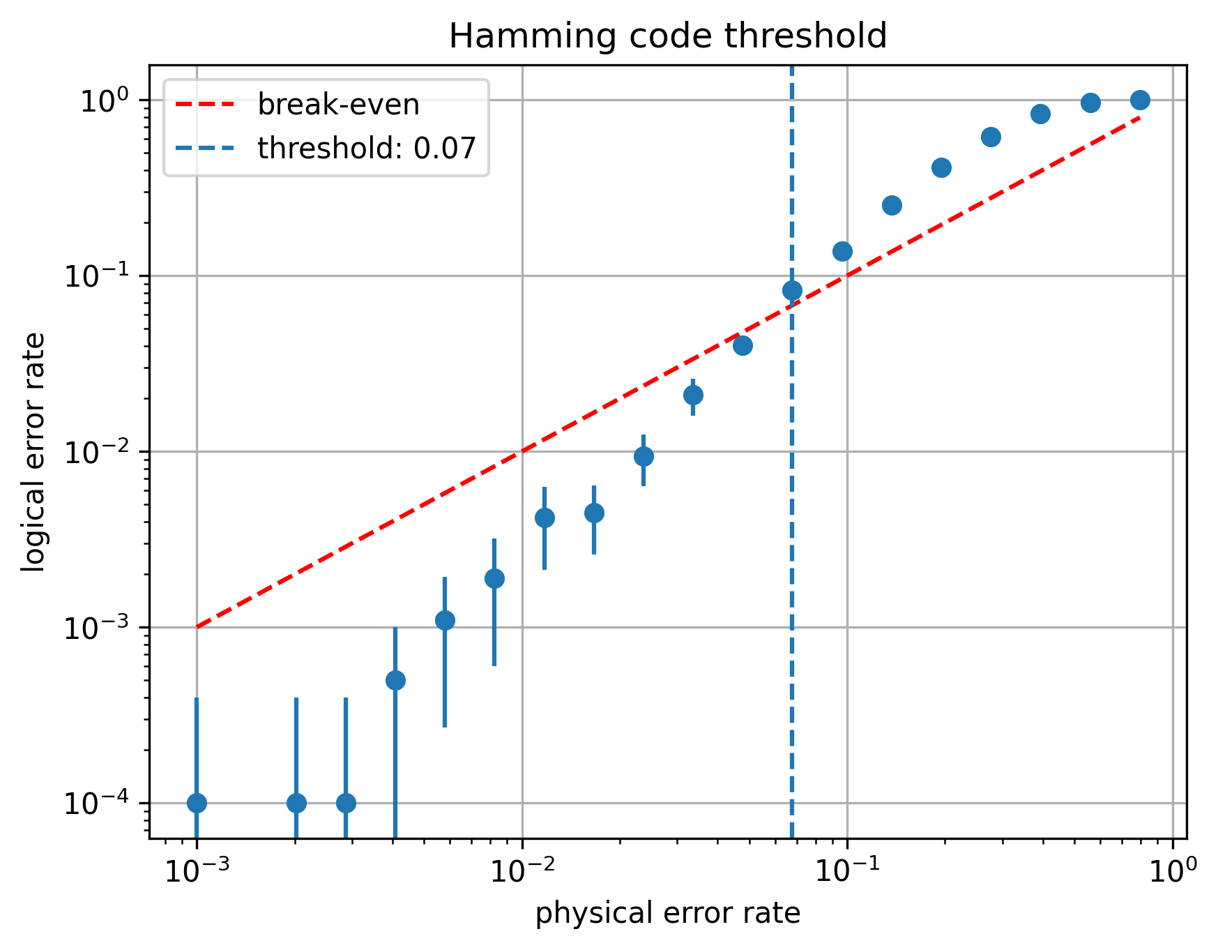

Next time

In the next post I will describe the Steane code, which can be thought of a quantum extension of the Hamming code described here. Many of the same ideas will reappear in the guise of quantum states and stabilizers, and we will end by approximating the break-even point of the Steane code.